LIFE, Zarr and everything

The LIFE metric maps the change in expected species extinctions per square kilometre when land is converted from one use to another. Our v1.01 release from the 2024 LIFE paper has been available from Zenodo in GeoTIFF format for a while now, but it was a little hard to use as this required downloading the whole TIFF and manually piping it into a workflow.

I've converted LIFE into into a streamable Zarr v3 store, and uploaded it to source.coop/tessera/life where it's served on the big cloud in the datacentre sky. The values here are the same as the Zenodo data, but now easily streamable over HTTP instead of downloading the whole archive. To make it easy to use this from your language of choice, we also now have LIFE.js, LIFE.py and LIFE.r available.

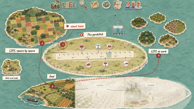
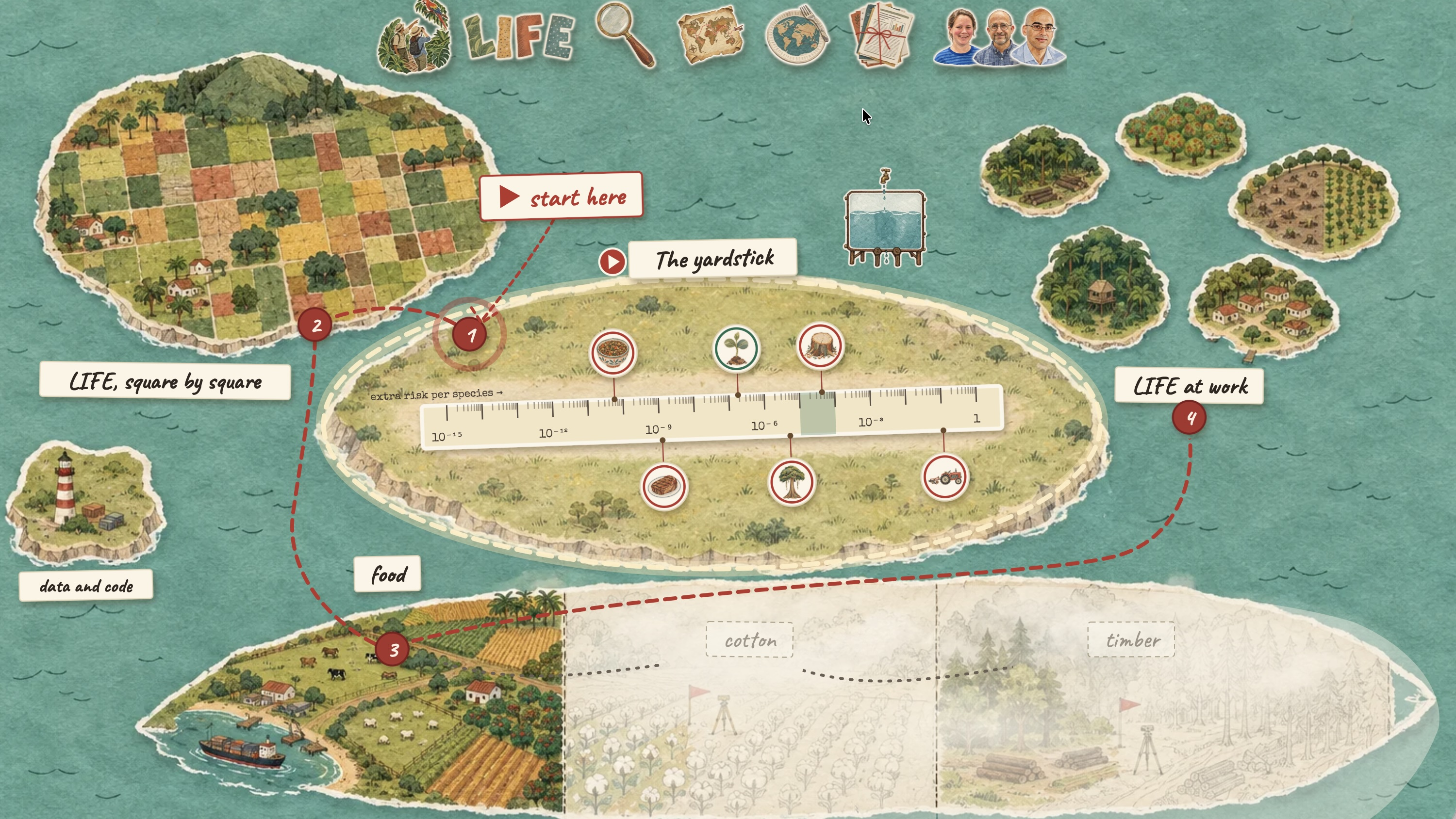
I also experimented with vibespiling with modern agents. I also used an ensemble of frontier agents to build an experimental 'interactive LIFE' guided tour, which blends real data from the Zarr with explanations of what's going on. The tour is still evolving and not a replacement for the official site, but I figured I'd open it up for feedback since the design capabilities of modern AI have come along remarkably since I last tried it a few months ago. I'm still on the fence whether I 'like this' or not vs a human narration, but there's no question that the production values of these models are incredible now. Listen to the tour above with your audio on!

1 What Zarr got to do with it?

Zarr is a format for chunked, compressed N-dimensional arrays, served in such a way that ordinary static HTTP hosting can serve it all. I've also picked this up for TESSERA in previous work, so it made perfect sense to also expose our other research datasets like this as well. A LIFE Zarr store is a simple tree of keys:

Each layer name in LIFE has a "scenario" and a "extinction curve". The scenario is the land-use change that's being modelled; arable converts remaining natural habitat to cropland, while restore returns land back to natural vegetation. The curve is a sensitivity-analysis parameter for the persistence-score function behind the metric; 0.25 is the main published result, and the other curve values exist to show how sensitive that result is. Most users will use 0.25.

https://source.coop/tessera/life/
  v1.01/
    zarr.json                     # root group with attributes and consolidated metadata
    0/                            # resolution level 0 (native, 1/60 degree)
      arable_0.25/
        zarr.json                 # shape, dtype, chunk shape, codecs
        c/2/5/13                  # one chunk: (taxon 2, chunk row 5, chunk column 13)
    1/ 2/ 3/ 4/                   # each level averages 2x2 blocks of the last

There are three kinds of files here. First, the zarr.json stores metadata for each group. E.g. 0/arable_0.25/zarr.json defines the array as having the dimensions [5, 10800, 21600] (taxon, latitude, longitude), that it's a float32, and is divided into [1, 1024, 1024] chunks, and that each chunk is zstd compressed. The root zarr.json is large because it also stores the consolidated metadata, so a client can investigate the whole store in a single HTTP request. Second, each file is a "chunk" that holds a compressed 1024×1024 tile of one LIFE band. A Zarr client can do the array math to find which chunks cover a region, and can fetch just those. Third, there are entries in the Zarr root attributes that declare proj:, spatial: and multiscales conventions, which give hints to Zarr clients about how to interpret the metadata (in this case, as a map projection).

As an example, reading Madagascar's LIFE scores (43°E 26°S to 51°E 12°S) for birds involves a client doing the following on the network:

1. HTTP GET zarr.json once, and read the grid: 10800×21600 pixels at 1/60°.
2. Calculate the array window (rows 6120–6960 and columns 13380–13860)of the base level, and that the birds are band 2 from the taxa list (all, AMPHIBIA, AVES, etc).
3. HTTP GET the chunk rows involved (0/arable_0.25/c/2/5/13 and c/2/6/13 in this case).
4. Decompress, crop and return an in-memory 840×480 array with the results.

That's about a megabyte of content, which is pretty good vs downloading a multi-gigabyte store from Zenodo with the GeoTIFFs. Because this dataset is relatively small overall compared to Tessera's bulk, the LIFE store doesn't use the sharding codec and so is much simpler.

2 The interactive tutorial

Once I'd transcoded the Zarr store, I built an 'ensemble' of agents in order to design a 'one shot' walkthrough to explain what LIFE does. The main inputs to it were the academic papers we've published over the last few years: the original LIFE paper, five ways to use it, and the food paper quantifying what we eat costs in extinctions.

The process was pretty simple:

1. I gave the model a brief about what I wanted in about a paragraph, requesting a 'whimsical, hand-drawn style'. I supplied the papers locally and then fact-checked the script that resulted, making only minor changes.
2. Generate the media. The Opus 5.5 model selected an ensemble of models and recorded the narration, scored the music, and generated the image cut-outs.
3. Animate in JavaScript. Each film is a JavaScript function (a pure function of time) rendered in the browser.
4. Mix the sound. Sound cues that were recorded earlier are placed beside the visuals, with the model generating some Python code to act as a static sound mixer and output keyframes to the JavaScript.
5. Review and render. A 'judging panel' of agents reviewed the mixed ensemble and rejected obviously bad ones with overlaps and so on.
6. Build the site. The LIFE metric site is a GitHub pages that serves it all, optimising the images and sound to use Web Audio.

This was a largely automated process! In the end, the models selected for each task were:

• Images: openai/gpt-image-2.5-flare painted the paper-collage cut-outs, textures, and the welcome painting and the team portraits.
• Narration: google/gemini-3.8-flash-tts with voice "Gacrux" did the narration.
• Music: google/lyria-3-pro-preview wrote the orchestral scores from the script briefs and a target length. This required several takes per film and a judging panel to discard mispronunciations and so on.
• Review: gemini-3.1-pro-preview helped rank voice and music takes, and its claims were checked against headless browser measurements, since it often hallucinated timestamps.
• Alignment: whisper then gave each narration individual word timings, which the JavaScript animation keys to for animation triggers.
• Code: Claude Opus 5.5 wrote the films, the engine and the site.

Total cost on OpenRouter was around £2 for all the models that weren't Claude (which I have on subscription). What I found a bit mindblowing is how powerful it is to have the streamable Zarr stores, as the coding model would dynamically query the data while forming the script in order to find interesting stories to tell from the paper, and then use them 'live' in the explanation via JavaScript.

3 Vibespiling the Zarr language bindings simultaneously

After this, I also vibespiled three separate client libraries in different languages. Since all three clients implement the same basic access to Zarr, it turns out to improve the quality of agentic generated code since they could cross-validate against each other and the reference implementation. The more languages I add in, the more edge cases were found!

3.1 LIFE in JavaScript

I put in a TypeScript layer here, as that's what the website tour above used.

import { open } from "life-metric";

const life = await open();
const raster = await life.read("arable_0.25", {
  bounds: [43, -26, 51, -12],   // west, south, east, north
  taxon: "AVES",
});
console.log(raster.width, raster.height, raster.units);

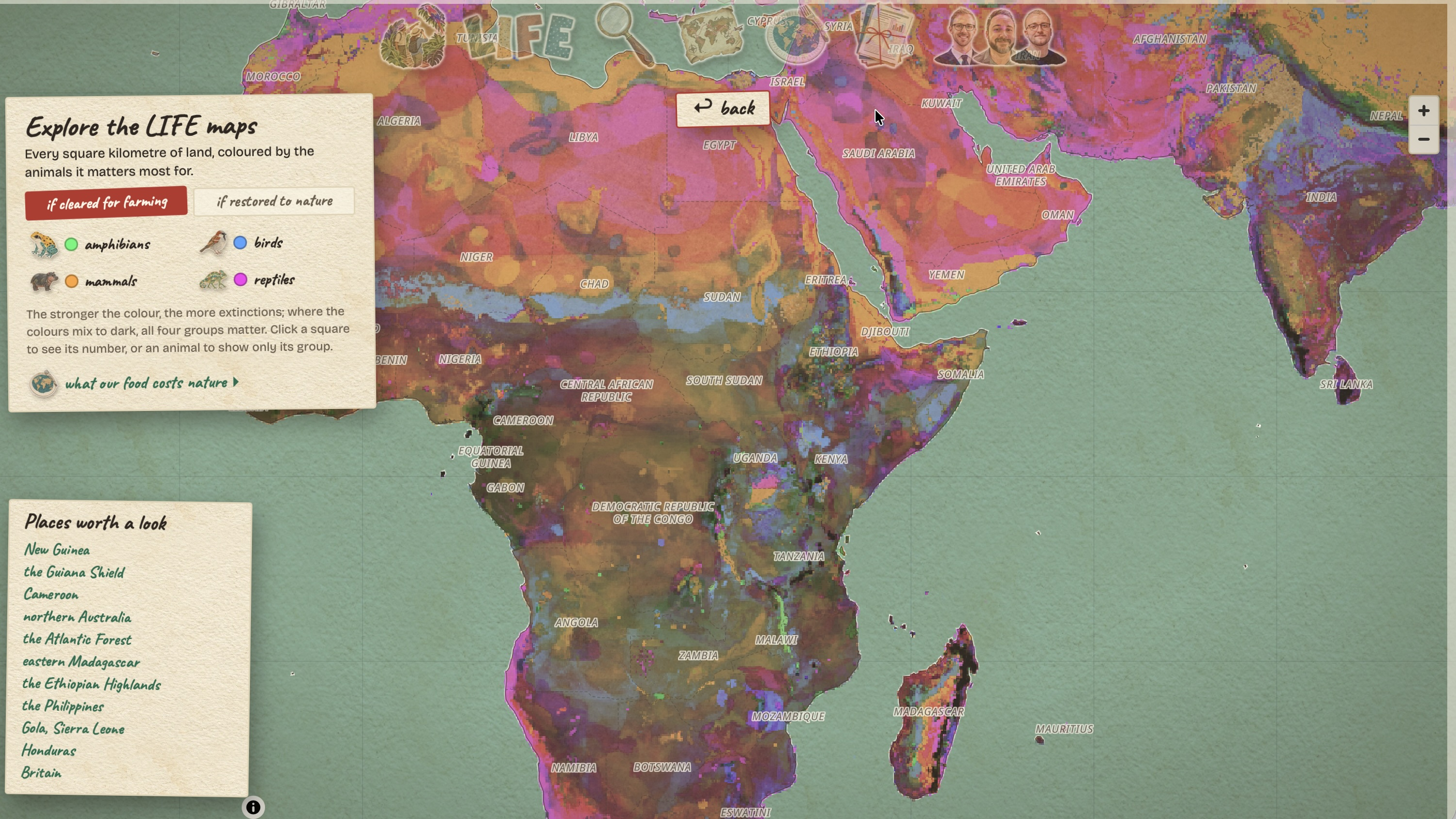
This works through zarrita to access Zarr, and works in both Node and in a browser. There aren't any masked arrays in JavaScript, so NaN handling needs to be done carefully. Cancellation is also carefully handled via an AbortSignal, so this'll work well in the MapLibre layer. The result is a LIFE globe viewer that is served straight from source.coop alongside the data.

3.2 Python

Michael Dales helped me figure out idiomatic interfaces for the Python client:

import numpy as np
from life_metric import read

values, transform = read("arable_0.25", taxon="AVES", bounds=(43, -26, 51, -12))
print(values.shape, np.nanmean(values))   # (840, 480) 1.5e-05

The first version that the agent wrote had its own custom BBox, Layer and Raster classes that looked reasonable, but that nobody who is already familiar with geospatial Python would have recognised! Michael Dales pointed library conventions to me, and the next iteration uses rasterio alongside an xarray/rioxarray path as well. This does make me think that having a 'awesome Python' style agent skill that lists reasonable library conventions would be useful to have.

3.3 R

Finally, the most requested language from ecologists is R, and so we have:

library(lifemetric)

life <- life_open()
birds <- life_read(life, "arable_0.25", bounds = c(43, -26, 51, -12), taxon = "AVES")
terra::global(birds, "mean", na.rm = TRUE)

The R client returns a terra SpatRaster, and reads the store with the native zarr package. However, I did have some trouble with sharded Zarr and so ensured our Zarr store was simply chunked. R also indexes arrays from one, which caught some indexing bugs in the generated code by cross-validating against the Python. Thomas Swinfield also explained to me how R packaging works and so I can publish this soon.

4 Closing (human) thoughts

The quality of the generated code in general was far, far higher than when I did my advent of agentic coding last December. However, the lack of a reference spec is still clearly a problem, as is the missing steer towards using existing libraries and idioms where possible. The cross-checking agentically was extremely effective given the numerical nature of the data... I'm also going to start integrating these layers with Shane Weisz into the Dash for Life to make it easier to cross-check species' AoHs with the global scores!

The packages will be published on PyPI, npm and R after I finish a few more rounds of manual review. In the meantime you can install each from its GitHub repository. The code I 'wrote' is MIT licensed, but the data is not: the LIFE data may not be used for commercial or revenue-generating purposes, nor redistributed in their original form, without written permission from our friends at IBAT ibat@ibat-alliance.org. By joining IBAT if you use this commercially, you will be helping to support the efforts of many people around the world working on assessing and collecting precious data on biodiversity across many thousands of species.